
Industry News
Curation by industry experts
Hot Articles
Popular Tags
How Is the Payback Period for Resource Recovery Equipment Calculated?
The payback period for resource recovery equipment is calculated by dividing the project’s net upfront investment by the annual net cash benefit it produces. The arithmetic is simple; the difficult part is defining the cash flows correctly. For an AI sorting line, pyrolysis unit, wastewater recovery system, or desalination asset, the purchase price alone says very little about investment recovery.
A credible calculation must capture the full cost of putting the asset into reliable operation and the incremental cash it creates or preserves after operating expenses. Recovered-material sales are only one possible benefit. Avoided landfill charges, lower freshwater purchases, reduced energy consumption, lower chemical demand, reduced discharge fees, and avoided compliance-related spending can be equally important. Conversely, power consumption, maintenance, consumables, residue handling, labor, financing structure, ramp-up losses, and downtime can materially lengthen the result.
The basic payback formula
For projects with relatively stable annual cash flows, simple payback is:
Payback Period (years) = Total Initial Investment ÷ Annual Net Cash Benefit
Where:
- Total Initial Investment is the cash required before commercial operation.
- Annual Net Cash Benefit is annual cash savings plus annual incremental revenue, minus annual incremental operating costs.
Expressed more fully:
Annual Net Cash Benefit = Recovered Resource Revenue + Avoided Costs + Incentives Received − Incremental Operating Costs
The calculation should be based on incremental cash flow: the difference between continuing with the current process and installing the recovery system. This distinction prevents a common error: crediting equipment with savings that would have occurred without the investment.
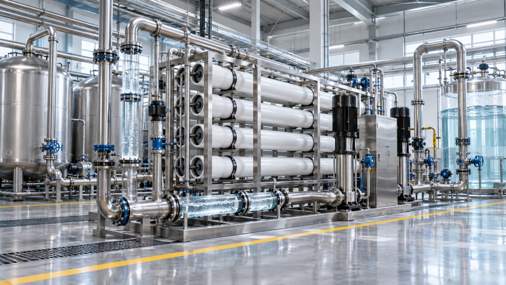
For example, a wastewater reuse system may reduce municipal water purchases and wastewater discharge volumes. The relevant benefit is not the gross value of all reused water; it is the actual reduction in water and discharge expenditure compared with the existing operating arrangement, after considering the electricity, membranes, chemicals, labor, concentrate disposal, and maintenance needed to produce that reuse water.
What belongs in the initial investment?
Supplier quotations often cover only the core equipment package. Payback calculations should instead use the installed, ready-to-operate cost. Depending on the technology and site, this may include:
- Equipment purchase price, freight, insurance, duties, and applicable taxes;
- Civil works, foundations, buildings, drainage, utility connections, and electrical upgrades;
- Engineering, process design, automation integration, commissioning, performance testing, and operator training;
- Feedstock preparation, conveyors, storage, odor control, emissions controls, brine or residue management, and fire protection where required;
- Permitting, environmental studies, inspections, and third-party certification costs;
- Initial spare parts, startup chemicals, membrane inventory, catalysts, or other critical consumables;
- Working capital needed for inventory, receivables, and startup operations; and
- Contingency for site-specific scope that is not yet technically defined.
The inclusion of indirect costs is especially important in resource recovery projects because the interface with the existing plant can be more expensive than the main process unit. A sorting system may require feed conditioning and downstream bale handling. A pyrolysis process may require drying, emission controls, char handling, and product storage. A desalination or industrial reuse plant may require intake, pretreatment, post-treatment, pipelines, and concentrate disposal infrastructure.
If the calculation excludes these costs, it does not represent the payback period of the project. It represents only the payback of a selected equipment package.
How annual benefits should be measured
Annual benefits should be built from physical operating assumptions before they are converted into currency. This is more reliable than starting with a desired financial outcome. The operating model normally begins with throughput, recovery rate, product yield, availability, product quality, unit prices, and avoided-cost rates.
For a material recovery facility, annual recovered-material revenue may be estimated as:
Annual Revenue = Feed Throughput × Recoverable Fraction × Recovery Rate × Saleable Quality Rate × Net Realized Price
The net realized price should account for sorting specifications, contamination deductions, moisture, transport to the buyer, brokerage costs, and any processing required before sale. A published commodity benchmark is not necessarily the price available at the facility gate.
For a wastewater recovery unit, the equivalent value of recovered water may be calculated from displaced water purchases and avoided wastewater charges. If reuse water replaces a lower-cost source, its value should be based on that source’s tariff, not on the tariff for premium potable water. If recovered water can only be used intermittently because plant demand is variable, the benefit must reflect actual usable volume rather than design capacity.
For thermal recovery and pyrolysis systems, benefits can involve fuel displacement, oil or gas sales, recovered carbonaceous solids, avoided disposal charges, and, in some configurations, recovered heat. Each revenue line requires a technically supportable yield and a commercially achievable offtake route. A theoretical product yield does not equal saleable output when the product requires upgrading, testing, blending, or market qualification.
Avoided disposal cost is often an important component, but it should be treated carefully. The avoided amount is the actual all-in disposal cost no longer paid: gate fees, transport, handling, taxes, and associated treatment charges. It is not a notional “environmental value” unless a contractual or regulated mechanism turns that value into cash.
Operating costs are where optimistic payback models fail
The annual operating-cost estimate should reflect normal operating conditions, not only nameplate performance. Relevant categories vary by technology but commonly include electricity, fuel, water, chemicals, membranes, media, catalysts, labor, laboratory testing, routine maintenance, replacement parts, insurance, monitoring, product transport, and residue disposal.
Energy should be modeled from expected specific consumption at the actual duty point. A system operating at partial load, treating a more difficult feed, or handling seasonal variations may use materially different energy per tonne or per cubic meter than a nominal datasheet figure suggests.
Maintenance costs also need a realistic boundary. Routine servicing, wear parts, planned shutdowns, and major periodic replacements are not interchangeable. In reverse osmosis applications, membrane replacement and pretreatment performance can be central to lifecycle economics. In sorting lines, wear components, optical sensor maintenance, compressed air demand, and belt-related downtime affect available processing hours. In thermal systems, refractory, feed preparation, emissions-control consumables, and residue management can be decisive.
Where a major replacement is expected after several years, simple payback may not show its effect adequately. It should still be disclosed in the model and assessed through lifecycle measures such as net present value (NPV), internal rate of return (IRR), or levelized treatment cost.
A worked example using illustrative figures
Assume an industrial facility is evaluating a water recovery unit. The figures below are hypothetical and intended only to show the calculation method.
- Installed equipment, integration, commissioning, and startup cost: US$2.4 million
- Annual savings from lower freshwater purchases: US$720,000
- Annual avoided wastewater discharge cost: US$280,000
- Annual electricity, chemicals, labor, maintenance, and concentrate-management cost: US$400,000
The annual net cash benefit is:
US$720,000 + US$280,000 − US$400,000 = US$600,000
The simple payback is therefore:
US$2,400,000 ÷ US$600,000 = 4 years
This four-year result is useful only if the benefits are achievable under the facility’s actual production profile. If the plant runs below forecast volume, if recovered water has limited reuse demand, or if the unit’s availability is lower during the first operating year, annual benefit will be reduced and payback will extend.
A more realistic model may use monthly or yearly cash flows rather than a single annual average. Suppose the project generates only 60% of its normal benefit in the first year because commissioning and process optimization take time, then reaches full benefit in year two. Cumulative payback occurs later than a model that assumes full performance from day one.
When annual cash flows vary, use cumulative payback
Many recovery projects do not generate identical annual benefits. Commodity prices move, utility tariffs change, disposal contracts are renegotiated, feedstock composition shifts, and major maintenance events occur. In these cases, calculate cumulative net cash flow period by period.
Start with the negative initial investment. Add the net cash benefit for each month, quarter, or year. The payback date is the point at which cumulative cash flow becomes positive.
If cumulative cash flow is still negative at the end of year three but becomes positive during year four, a fractional payback period can be estimated as:
Payback = Last Full Year Before Recovery + Remaining Unrecovered Investment ÷ Net Cash Benefit in the Recovery Year
For instance, if US$150,000 remains unrecovered after year three and year-four net cash benefit is forecast at US$600,000, the additional recovery time is 0.25 year. The payback period is 3.25 years.
This approach is preferable where seasonal feedstock, staged capacity increases, contract pricing, or commissioning schedules drive uneven performance.
Compliance benefits require a cash-flow test
Environmental compliance can have substantial economic importance, but it should not be treated as an automatic revenue line. The key question is whether the recovery system avoids a clearly identifiable cash outflow or enables continued lawful operation under a defined requirement.
Examples of potentially measurable compliance-related benefits include an avoided surcharge, avoided off-site treatment fee, avoided expenditure on an alternative control system, or avoided production interruption where the cost can be credibly established. Potential reputational gains, broad sustainability claims, and uncertain future penalties should not be inserted into a base-case payback calculation as if they were cash savings.
Carbon credits, renewable-energy certificates, recycled-content premiums, and government support may improve economics where eligibility, ownership, verification requirements, and payment timing are known. Their treatment should be conservative. If an incentive is provisional, competitive, transferable only under limited conditions, or dependent on future rulemaking, it is better assessed as an upside scenario rather than embedded in the base case.
Simple payback is not the final investment decision
Payback answers a narrow question: how long until the initial cash outlay is recovered? It does not measure the value created after that point, does not account for the time value of money, and does not distinguish between a durable asset and one with short-lived benefits.
A project with a shorter payback is not automatically the better project. One system may recover its investment quickly but have higher technical risk, greater exposure to volatile product prices, or limited strategic value. Another may have a longer payback but provide secure water supply, reduce dependence on constrained disposal capacity, improve permit resilience, or remain valuable for a much longer operating life.
For this reason, resource recovery projects are usually stronger when simple payback is reviewed alongside discounted cash flow metrics. NPV discounts future cash flows using the organization’s required return or cost of capital. IRR indicates the discount rate at which the project’s NPV equals zero. Scenario analysis tests whether the investment remains acceptable when key variables change.
The variables worth stress-testing are those that actually drive the economics: material or energy price, disposal cost, recovery yield, utility tariff, uptime, feed quality, throughput, consumable use, and product acceptance by downstream buyers. A model that changes every input by the same percentage can look sophisticated while missing the operational conditions that matter most.
Common calculation errors
The most frequent error is using nameplate throughput instead of confirmed feed availability. Equipment can only recover value from material, water, or energy that is consistently available and suitable for treatment. Design capacity should not be confused with annual processed volume.
Another is double counting. A project should not simultaneously claim the full sale price of a recovered material and the full avoided purchase cost of the same material unless both cash effects genuinely occur. The same caution applies to energy recovery, disposal avoidance, and compliance savings when the underlying cost is already included elsewhere.
Ignoring residual streams also distorts results. Recovery processes often create rejects, concentrates, spent media, ash, sludge, or contaminated fractions that still require treatment, transport, or disposal. These costs belong in the operating model.
Finally, calculations should state whether they are pre-tax or post-tax, nominal or real, and whether financing costs are included. Simple project payback is commonly presented on an unlevered, pre-tax basis so that technology economics can be compared independently of a buyer’s capital structure. If debt service is included, it should be labeled clearly because the result then reflects financing terms as well as project performance.
A defensible payback period starts with operational evidence
The most useful answer to “How do you calculate the payback period for resource recovery equipment?” is not a single formula but a traceable cash-flow model. Every major benefit should link to a physical basis, a commercial price or tariff, and an operating assumption. Every major cost should have an owner, a scope boundary, and a timing assumption.
When the model is built this way, payback becomes more than a headline number. It reveals which conditions must hold for the investment to work: the minimum throughput needed, the required recovery rate, the tolerated electricity cost, the buyer specification for recovered output, or the availability level needed to protect savings. Those are the conditions that determine whether a resource recovery project creates durable value rather than only an attractive spreadsheet result.
Recommended News
How energy recovery cuts the cost of seawater desalination in the Middle East
Seawater desalination Middle East projects can cut lifecycle costs with energy recovery. Explore savings, bankability, power-risk strategies, and smarter investment decisions.
What drives nuclear safety solutions pricing for new facility projects?
Nuclear safety solutions pricing explained: uncover the key cost drivers for new facilities, from qualification and interfaces to lifecycle support.
What drives radioactive waste cost over the life of a disposal project?
Radioactive waste cost depends on classification, treatment, transport, storage, disposal access, and long-term compliance. Explore the key lifecycle cost drivers.
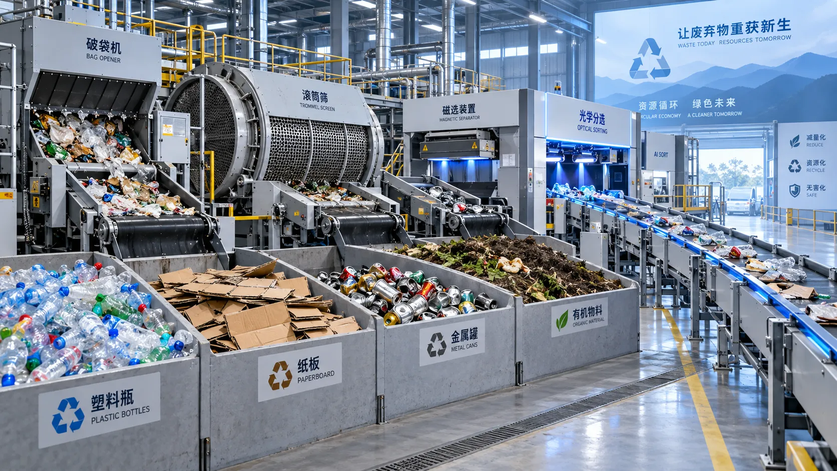
How to choose solid waste equipment based on waste stream characteristics
Environmental equipment guide for solid waste: discover how to match sorting, treatment, and recovery equipment to waste composition, moisture, contamination, and output goals.
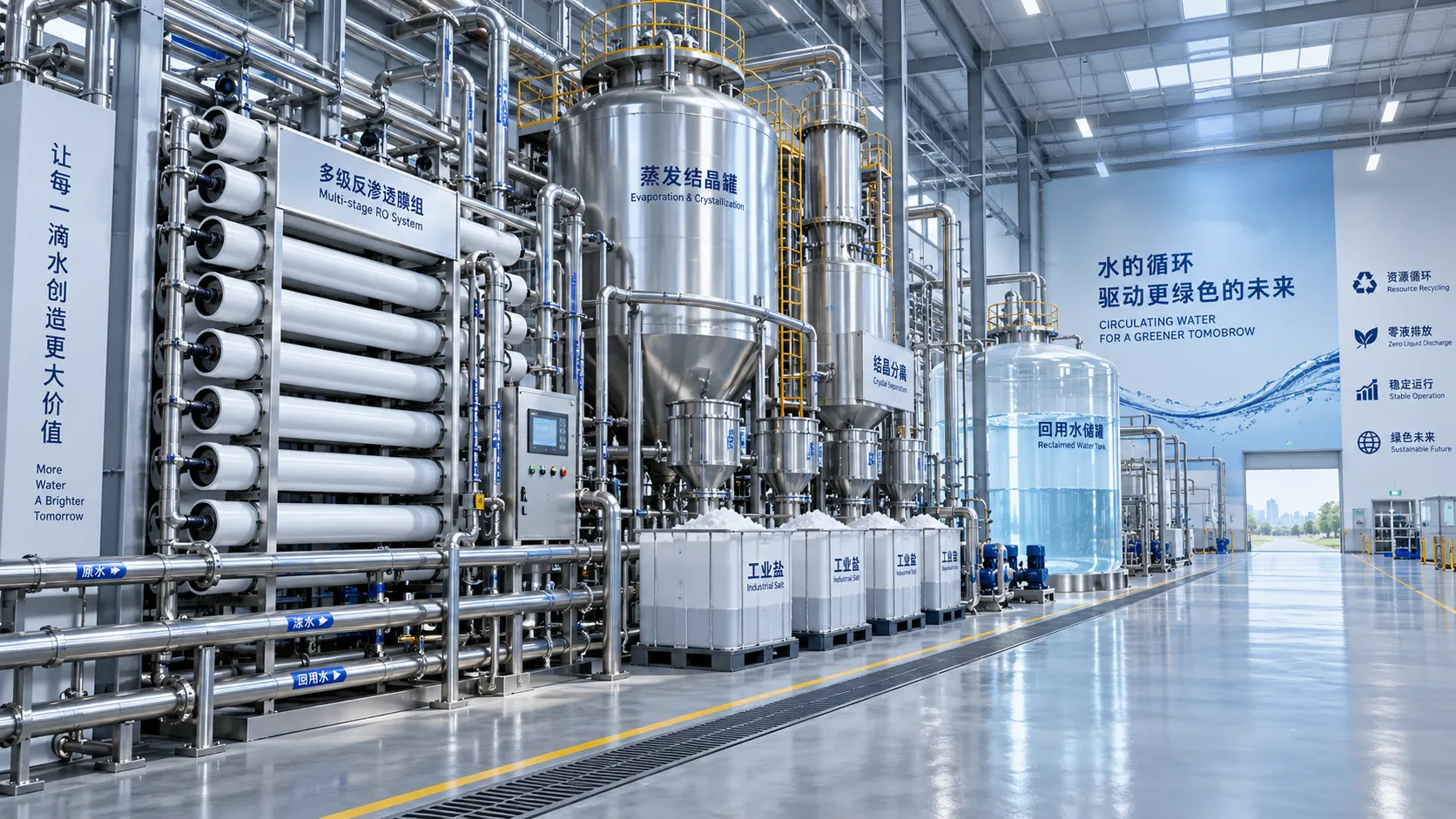
When does high recovery ZLD equipment justify its higher capital cost?
High recovery ZLD equipment can justify higher capital cost when water scarcity, discharge risks, brine disposal, and downtime threaten operations. Explore the decision factors.

How high purity heavy metal recovery affects recovered metal value
High purity heavy metal recovery boosts recovered metal value by improving payability, reducing penalties, and unlocking stronger buyer opportunities. Explore smarter netback strategies.
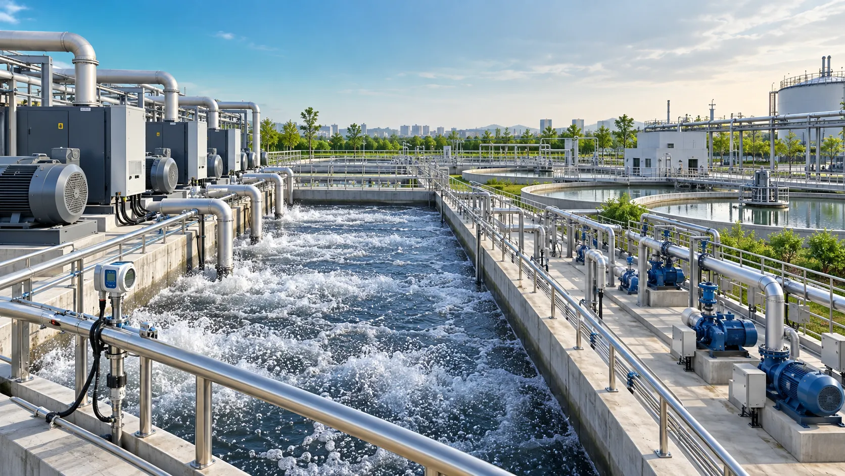
When does environmental equipment intelligence reduce wastewater plant energy use?
Environmental equipment intelligence for wastewater plants cuts energy use through smarter aeration, pumping, and data-driven controls—without compromising compliance. Discover when it delivers measurable savings.
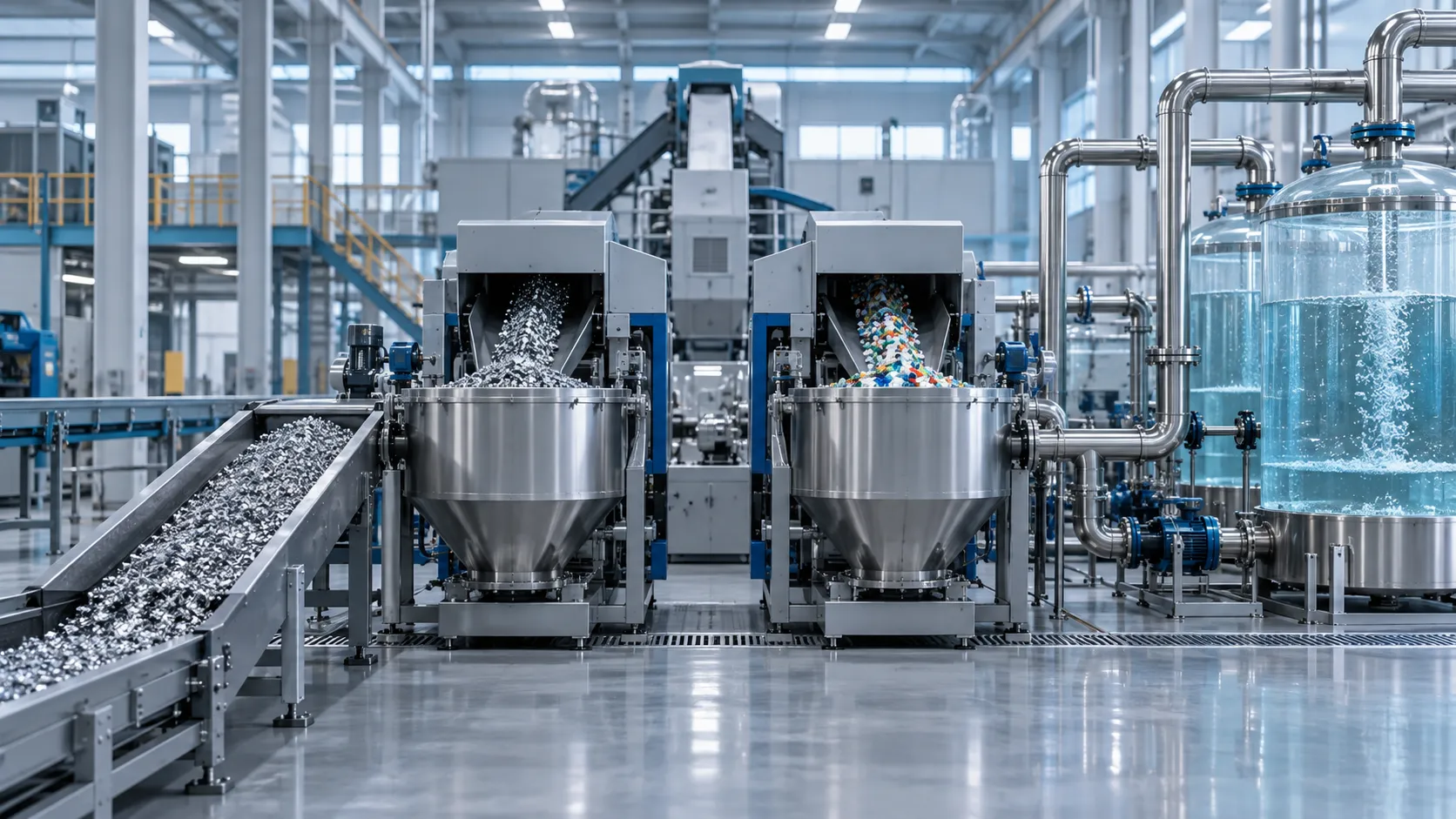
Which Circular Economy Model Is Best for Industrial Waste Recovery?
Which circular economy model works best for industrial waste recovery? Compare closed loops, industrial symbiosis, recycling, and energy recovery to choose the right strategy.
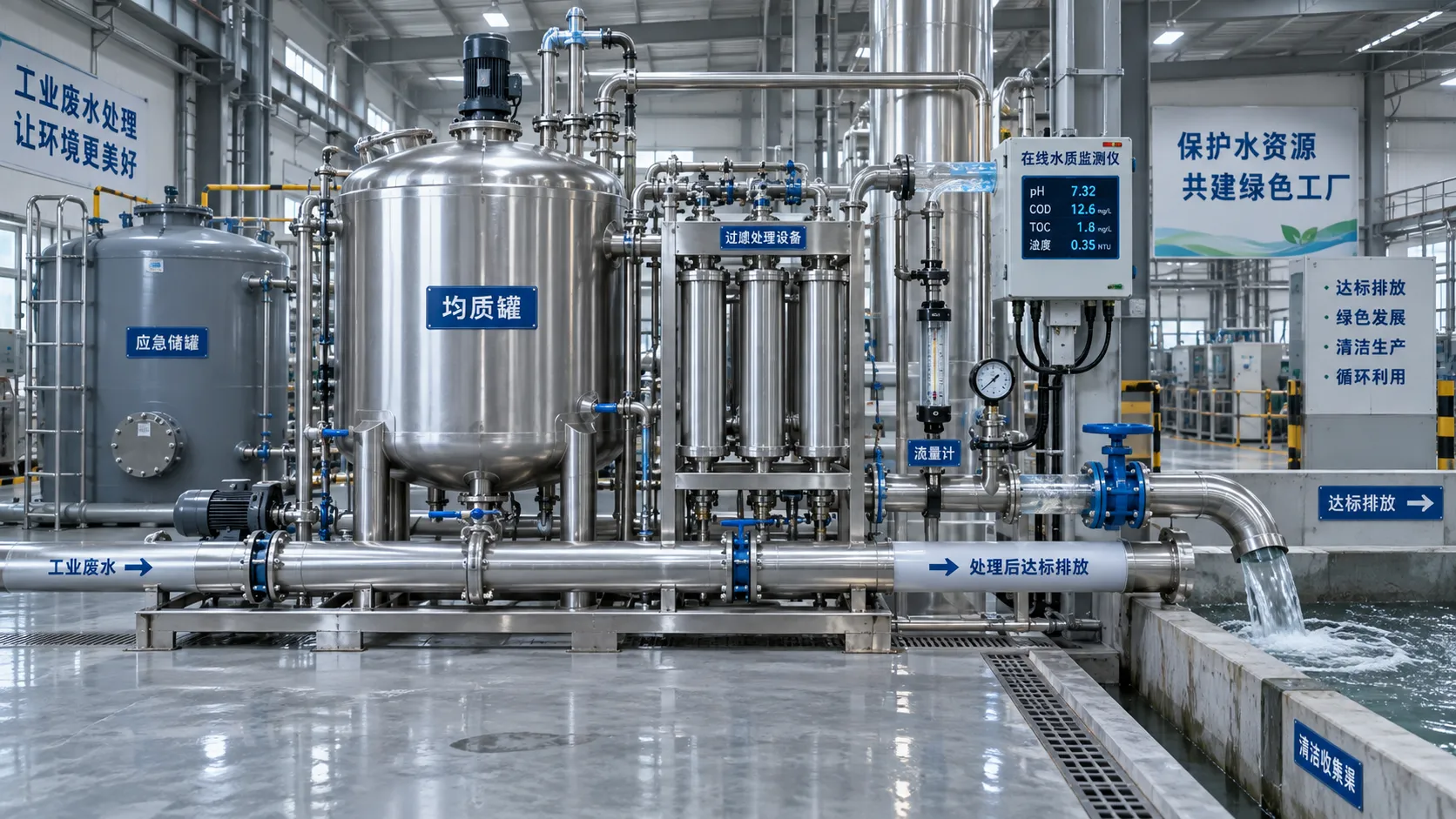
What Are the Main Compliance Risks in Industrial Wastewater Discharge?
What are the main compliance risks in industrial wastewater discharge? Explore permit exceedances, monitoring failures, hazardous contaminants, and practical controls to reduce liability.